Use case WF 6
Forecasting future phytoplankton dynamics using predictive models
Understanding and forecasting phytoplankton dynamics is essential for assessing aquatic ecosystem health, supporting conservation and management strategies, and anticipating potentially harmful algal blooms. Phytoplankton communities respond quickly to environmental fluctuations, such as changes in temperature, nutrient concentrations, hydrology, and light availability, making their behavior both highly dynamic and difficult to predict. For this reason, predictive modeling has become a key approach for capturing the complex, nonlinear, and often seasonal patterns that characterize long-term ecological time series. For this case study, we developed an analytical workflow to examine a long-term dataset of freshwater phytoplankton collected in Umbrian lakes from 2009 to 2022 and to explore different forecasting approaches aimed at gaining deeper insight into temporal phytoplankton dynamics. The workflow includes some of the most commonly used models for analyzing long-term ecological time series and generating forecasts, such as Random Forest, Support Vector Regression (SVR), and SARIMAX. These methods represent a combination of machine-learning and statistical approaches capable of capturing nonlinear relationships, seasonal patterns, and temporal dependencies. By applying and comparing these models, we aim to evaluate their predictive performance, identify key environmental drivers, and assess their suitability for forecasting future changes in phytoplankton communities.
Dataset used: Long-term dataset of freshwater phytoplankton in Umbrian lakes
The dataset includes:
- Phytoplankton Data Table: This dataset contains species density (cells/L) and biomass values expressed as biovolume (µm³/L) for each species collected between 2009 and 2022 with bi-monthly sampling.
- Abiotic Data Table: This table contains bi-monthly measurements of physico-chemical environmental parameters such as alkalinity, total nitrogen, total phosphorus, dissolved organic carbon, conductivity, dissolved oxygen, pH, depth, silica, water and air temperature, and transparency.
Data were collected from 9 sampling sites across 8 water bodies in the Umbria region during the monitoring activities carried out by ARPA Umbria, including 8 lakes: 2 natural lakes (Trasimeno and Colfiorito) and 6 heavily modified water bodies (HMWBs). Additional details about the dataset used in this use case are publicly available through the LifeWatch Italy metadata catalogue at the following link: https://metadatacatalogue.lifewatchitaly.eu/geonetwork/srv/eng/catalog.search#/metadata/18a16c1c-1296-47be-84f0-c27c7f1520f8.
Methods
Before the analysis, both the environmental and phytoplankton datasets were cleaned, standardised, and checked for inconsistencies. To facilitate the integration of biological and environmental information, the two datasets were then merged, ensuring that only observations collected simultaneously were retained. Each sampling month was also assigned to a climatic season (Winter, Spring, Summer, Autumn), and phytoplankton density values were aggregated at the monthly scale to reduce noise and highlight seasonal patterns. After merging the datasets, seven lakes were represented in the final table: Aia, Arezzo, Colfiorito, Corbara, San Liberato, Piediluco, and Trasimeno, while Lake Alviano was excluded because phytoplankton data for this site were not available. Exploratory analyses assessed the temporal behaviour of abiotic variables and the seasonal structure of phytoplankton density. Time-series plots were used to visualise environmental trends, boxplots described seasonal density distributions, and Pearson correlation matrices characterised relationships among abiotic predictors. Two modelling approaches were applied. First, static predictive models were used to estimate phytoplankton density from abiotic drivers. Density values were log-transformed to stabilise variance and reduce the influence of extreme bloom events. To avoid multicollinearity among predictors, only a selected subset of abiotic variables was included in the models: water temperature, conductivity, total nitrogen, total phosphorus, transparency, and dissolved oxygen. Temporal descriptors (year and month) and an autoregressive term (density_lag1) were also incorporated. Four machine-learning algorithms were tested: Linear Regression, Ridge Regression, Support Vector Regression, and Random Forest Regression. Model performance was evaluated using a 75/25 train–test split and quantified using R², MAE, and RMSE. To identify the most influential environmental drivers shaping phytoplankton dynamics, SHAP (SHapley Additive exPlanations) analysis was applied to the best-performing machine-learning models for Lake Trasimeno and Lake Piediluco. This approach provides model-agnostic and interpretable estimates of feature contribution by quantifying how each predictor shifts the model output relative to a baseline expectation. Second, a time-series forecasting framework was constructed using Seasonal ARIMA with exogenous variables (SARIMAX). Phytoplankton density and environmental variables were aggregated into bimonthly means, producing a regular 2-month time series for each lake. SARIMAX models were fitted on log-transformed density (log₁₀(density + 1)), and forecasts were back-transformed to the original scale for interpretation. Exogenous predictors were selected based on SHAP importance.
Results
Machine learning models and feature contributions
When all lakes were analysed together, Support Vector Regression and Random Forest achieved moderate predictive skill (test R² ≈ 0.34–0.44, Table 1), showing that global models can capture part of the common variability across systems when density is log-transformed and only weakly correlated abiotic variables are included. However, the global approach remained limited, as other algorithms returned near-zero or negative test R² values, confirming that strong ecological heterogeneity prevents effective generalisation. Model performance improved markedly when lakes were modelled individually, demonstrating that phytoplankton dynamics are predominantly lake-specific. The highest predictability was observed in Lake Trasimeno and Lake Piediluco. In Trasimeno, SVR reached a test R² of ~0.45 and Random Forest ~0.39, with low MAE and RMSE values indicating accurate reproduction of seasonal patterns and limited influence of extreme peaks. Piediluco showed similarly strong performance: Ridge Regression and SVR produced test R² values of ~0.44 and ~0.38, and MAE and RMSE remained close, suggesting stable dynamics and the absence of large, unpredictable bloom events. In contrast, lakes such as Aia, San Liberato, Colfiorito and Arezzo exhibited substantially lower predictive skill, with RMSE far exceeding MAE, reflecting sharp and irregular phytoplankton fluctuations that the models were unable to anticipate. Overall, the joint interpretation of R², MAE and RMSE shows that lake-specific modelling considerably outperforms the global approach, and identifies Trasimeno and Piediluco as the most predictable systems, providing the strongest basis for subsequent SARIMAX forecasting.
Table 1. Machine learning performance for Linear regression, Ridge Regression, Support Vector Regression, and Random Forest Regression model for each lake.
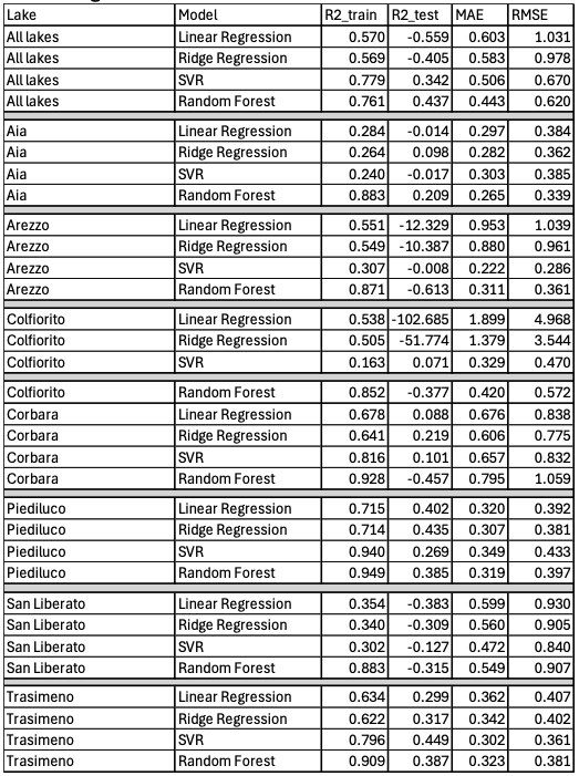
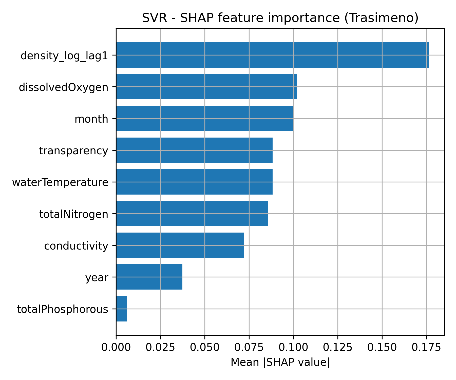
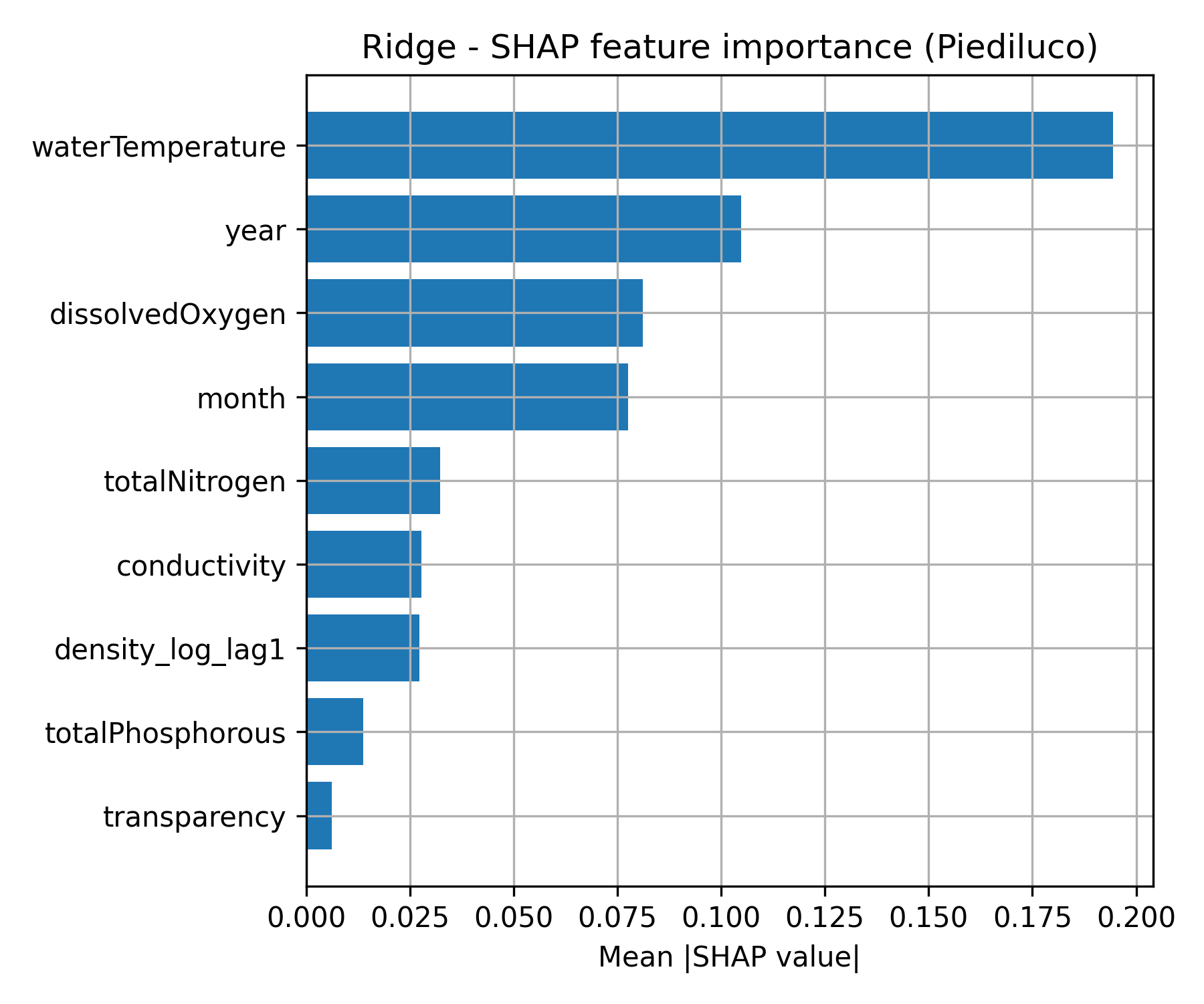
Figure 1. SHAP feature importance for the best-performing machine learning models at a) Lake Trasimeno (SVR; left) and b) Lake Piediluco (Ridge Regression; right).
Sarimax Forecasting Machine learning models
For Lake Trasimeno (Figure 2a), the observed density time-series is characterized by recurrent seasonal peaks throughout 2009–2022, but with relatively low magnitudes and a clear contraction in peak amplitude after 2016–2017. In the most recent years, densities drop to exceptionally low levels with only weak seasonal pulses, indicating a progressive suppression of phytoplankton dynamics. The SARIMAX model incorporates this attenuation, generating short-term forecasts that remain close to the historically low values while showing widening confidence intervals over the forecast horizon. This reduced predictability is consistent with the diagnostic results: the Ljung–Box test shows only weak evidence of residual autocorrelation at lag 20 (p ≈ 0.10), suggesting that the main temporal structure is captured despite the recent regime shift. For Lake Piediluco (Figure 2b), phytoplankton density shows a contrasting behaviour. The seasonal cycle remains well defined across the entire time-series, but from around 2016 onward the amplitude of seasonal peaks increases markedly, approximately doubling compared to earlier years, indicating stronger phytoplankton pulses without a clear long-term trend. This regular yet intensified seasonal dynamic is effectively reproduced by the SARIMAX model, whose forecasts follow the established pattern and display only a gradual expansion of uncertainty. The Ljung–Box test confirms an adequate model fit, with no significant residual autocorrelation at lag 20 (p ≈ 0.90), consistent with residuals behaving as white noise.
Overall, the two lakes exhibit contrasting temporal trajectories: a declining and increasingly subdued phytoplankton dynamic in Lake Trasimeno versus a stable but intensifying seasonal pattern in Lake Piediluco. In both cases, the SARIMAX models successfully reflect these underlying dynamics, projecting the observed tendencies into the forecast horizon with appropriate levels of uncertainty.


Figure 2 SARIMAX forecasts of phytoplankton density for a) lake Trasimeno and b) lake Piediluco. Observed densities (blue) and 3-year forecasts (orange dashed) with 95% confidence intervals (shaded).
Technical Notes
The entire modelling workflow can be applied either to each lake individually, allowing lake-specific dynamics to be characterized or to the combined dataset including all lakes, enabling the identification of broader, system-level patterns across the region. Although this case study focused on phytoplankton density, the workflow can be easily adapted to model other key parameters or used in other ecosystems.