Use case WF 5
Spatial and temporal distribution patterns of phytoplankton from Mediterranean and Black Sea lagoons
Transitional waters comprise diverse and dynamic ecosystems, including lagoons, estuaries, coastal lakes, salt marshes and salt pans. Their heterogeneity arises from geomorphology, catchment geology, freshwater inputs, tidal exchanges, climatic variability and human activities, all of which contribute to habitat complexity and shape ecological responses. Phytoplankton communities in these systems are highly sensitive to natural gradients and anthropogenic pressures, displaying distinct spatial and temporal patterns and specific morphometric adaptations. The present workflow was developed to analyse phytoplankton guilds across a set of transitional ecosystems in the eastern Mediterranean region, with the aim of identifying spatial and seasonal patterns in species richness, abundance and taxonomic composition, and of exploring how the structural traits of phytoplankton guilds relate to key hydrological, physico-chemical, climatic and physiographic variables.
Dataset used: Individual level trait-based dataset of phytoplankton communities from the coastal lagoons of the Mediterranean and Black Sea
The dataset consists of 104,687 individual phytoplankton records collected at 14 sites and 55 stations across five countries of the northern Mediterranean and western Black Sea (Albania, Bulgaria, Greece, Italy and Romania). The data were generated within the INTERREG IIIB TWReference Net Project and harmonized according to FAIR principles. The dataset consists of:
- Phytoplankton Morphological Trait Dataset – individual-based records of cell morphology, shape, size, density, biovolume, carbon content and biomass.
- Abiotic Dataset – Measurements of salinity, conductivity, temperature, pH, dissolved oxygen, total dissolved solids, and nutrient concentrations (NO₂, NO₃, NH₄, PO₄, SiO₂) and main physiographic and hydrological characteristics of studied transitional waters.
The study sites represent microtidal, nutrient-rich lagoon ecosystems that differ in their environmental characteristics and degrees of human impact. Additional details about the dataset used in this use case are publicly available through the LifeWatch Italy metadata catalogue at the following link: https://metadatacatalogue.lifewatchitaly.eu/geonetwork/srv/eng/catalog.search#/metadata/664e8015-1a16-4fff-82f9-7904e5b42226.
Methods
All analytical steps developed for this case study are summarised in Figure 1. A preliminary cleaning and filtering step was performed as a quality control measure to exclude localities lacking density or other trait information. For each sampling point, total cell density, species richness and diversity indices were computed. Species-level abundance data were log₁₀(x+1) transformed, and a sample × species matrix was used for multivariate analyses. Spatial and seasonal variation in phytoplankton density and richness was assessed using analysis-of-variance models, including two-way ANOVAs with locality and season or country and season as fixed factors, as well as a nested ANOVA with localities nested within countries
Sampling points were treated as replicates. Homogeneity of variances was assessed using Levene’s test, and normality of residuals was evaluated using Shapiro–Wilk tests. Relationships between species richness and log-transformed cell density were analysed at two spatial scales. At the sample level, Pearson correlations and simple linear regressions were fitted using all individual sampling points. At the ecosystem scale, mean richness and mean cell density were computed for each locality × season combination, and Pearson correlations and linear regressions were conducted using these aggregated values. Patterns in community composition were described using the sample × species abundance matrix, from which Bray–Curtis dissimilarities were calculated. Morisita–Horn similarity was computed to quantify taxonomic similarity among ecosystems. Multivariate structure was visualised using non-metric multidimensional scaling (nMDS) based on Bray–Curtis distances; ecosystem centroids were used to highlight group-level patterns. SIMPER analysis was applied to determine the taxa contributing most to compositional differences among ecosystems. To investigate environmental controls on phytoplankton structure, relationships between individual physicochemical and physiographic variables and phytoplankton metrics (density, richness, and taxonomic similarity) were examined through univariate ordinary-least-squares regressions. Abiotic heterogeneity among ecosystems was quantified by computing Euclidean distances from square-root transformed environmental variables. Environment–community coupling was evaluated using a Mantel-type correlation comparing Bray–Curtis dissimilarity with environmental distances. A multiple regression approach based on forward stepwise selection (p-entry = 0.05) was then used to identify the strongest combination of predictors for mean density and mean richness.Model performance was assessed using adjusted R² and F-statistics.
Results
Spatial and seasonal variation in phytoplankton density and richness
After a preliminary filtering step that excluded localities lacking density information, the analyses were carried out on a total of 263 samples collected from 12 coastal lagoons across five countries (Albania, Bulgaria, Greece, Italy and Romania) and during two seasons (spring and autumn). Total number of records are 83841 among 8 phyla, 20 classes, 95 families, 127 genera and 223 species. Phytoplankton density exhibited marked spatial heterogeneity across the twelve coastal lagoons (Figure 1a). The two-way ANOVA confirmed a strong locality effect (F₁₁,₂₃₉ = 642.24, P < 0.001) and a significant but smaller seasonal effect (F₁₁,₂₃₉ = 33.16, P < 0.001), with a significant locality × season interaction (F₁₁,₂₃₉ = 17.05, P < 0.001). Autumn samples generally displayed higher densities than spring samples, although the magnitude and direction of seasonal differences varied among lagoons. The highest densities were observed in Lehaova and Sinoe, both exceeding log₁₀(density) ≈ 7, while the lowest values occurred in Logarou and Aghios Nikolaos, where most samples remained below log₁₀(density) ≈ 4.5. Several lagoons (e.g. Karavasta, Varna, Margherita di Savoia) showed limited seasonal shifts, whereas others (e.g. Logarou, Narta) exhibited clear spring–autumn contrasts. Mean cell densities spanned almost four orders of magnitude. The lowest mean density was observed in Logarou lagoon in spring (5.9×10³ cells L⁻¹ on average; 2.3×10³–1.1×10⁴ cells L⁻¹,), whereas the highest mean density occurred in Lehaova lagoon in autumn (1.78×10⁷ cells L⁻¹ on average; 1.57×10⁷–2.02×10⁷ cells L⁻¹). Patterns of species richness mirrored these spatial differences (Figure 1b). Lagoons such as Lehaova and Sinoe consistently supported the richest assemblages, often exceeding 20 taxa per sample, whereas Patok, Logarou and Narta showed much lower richness, frequently below 10 taxa. Seasonal differences were less consistent than for density: some lagoons (e.g. Varna, Aghios Nikolaos) showed higher richness in spring, whereas others (e.g. Lehaova, Karavasta) displayed comparable values across seasons. Across individual samples, species richness was positively correlated with phytoplankton density (Pearson r = 0.538, p < 0.0001) (Figure 2a). Despite substantial scatter, particularly at intermediate densities, the overall trend was clearly increasing, consistent with the significant linear relationship (r = 0.538, P < 0.0001). At the ecosystem scale (locality × season, n = 24), this relationship became stronger (Pearson r = 0.703, p = 0.0001) (Figure 2b). Mean richness increased linearly with phytoplankton density (y = 3.68x – 8.66), indicating that ecosystems with higher phytoplankton density also supported more diverse assemblages (Figure 2 a, b).
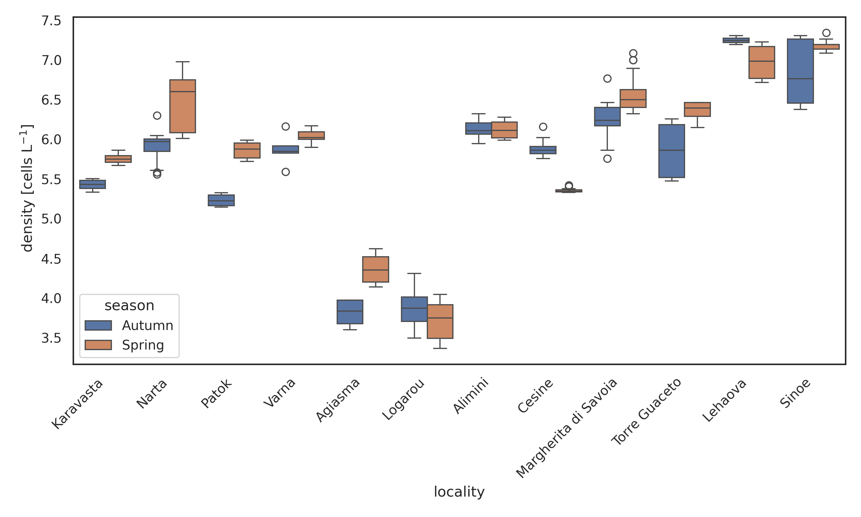
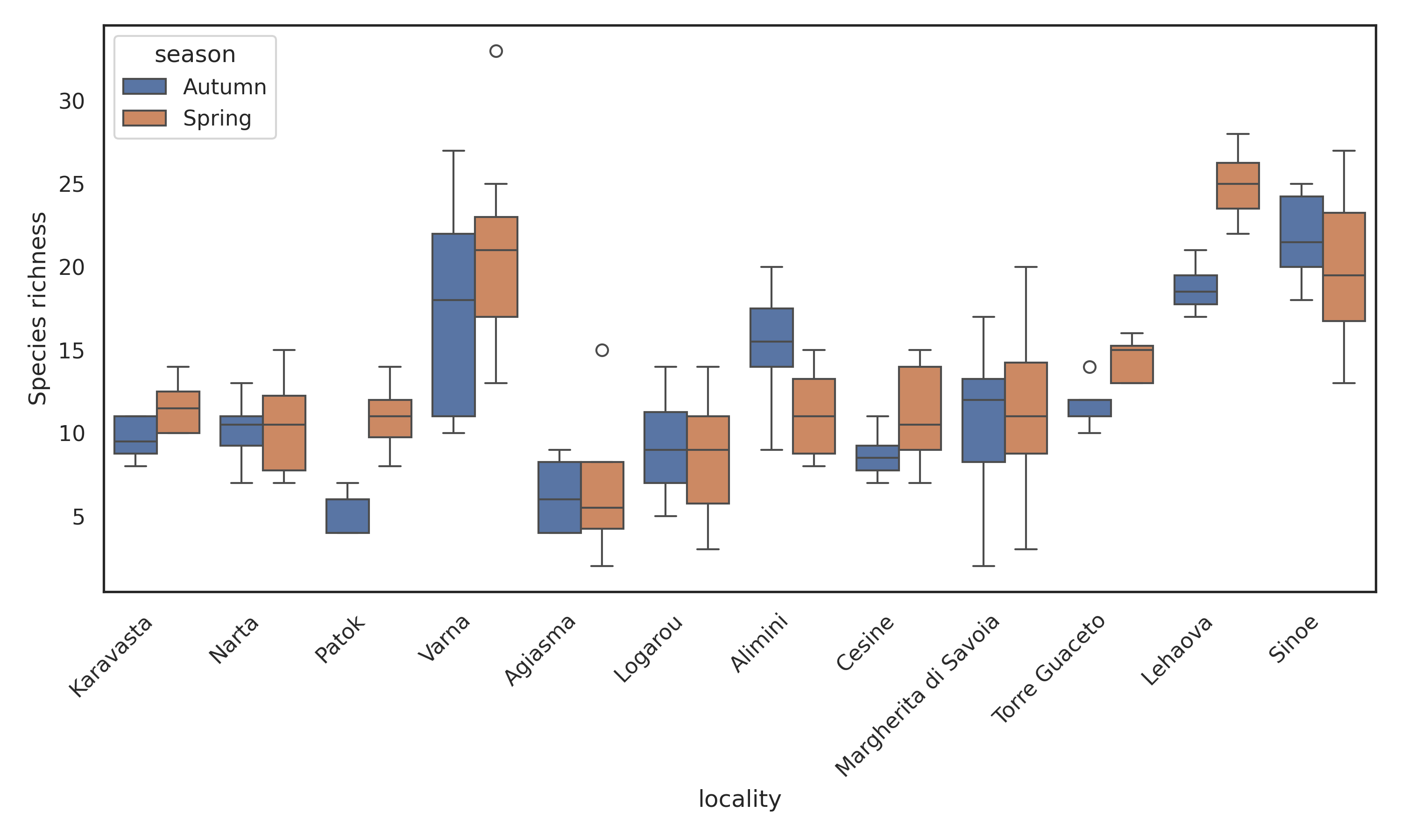
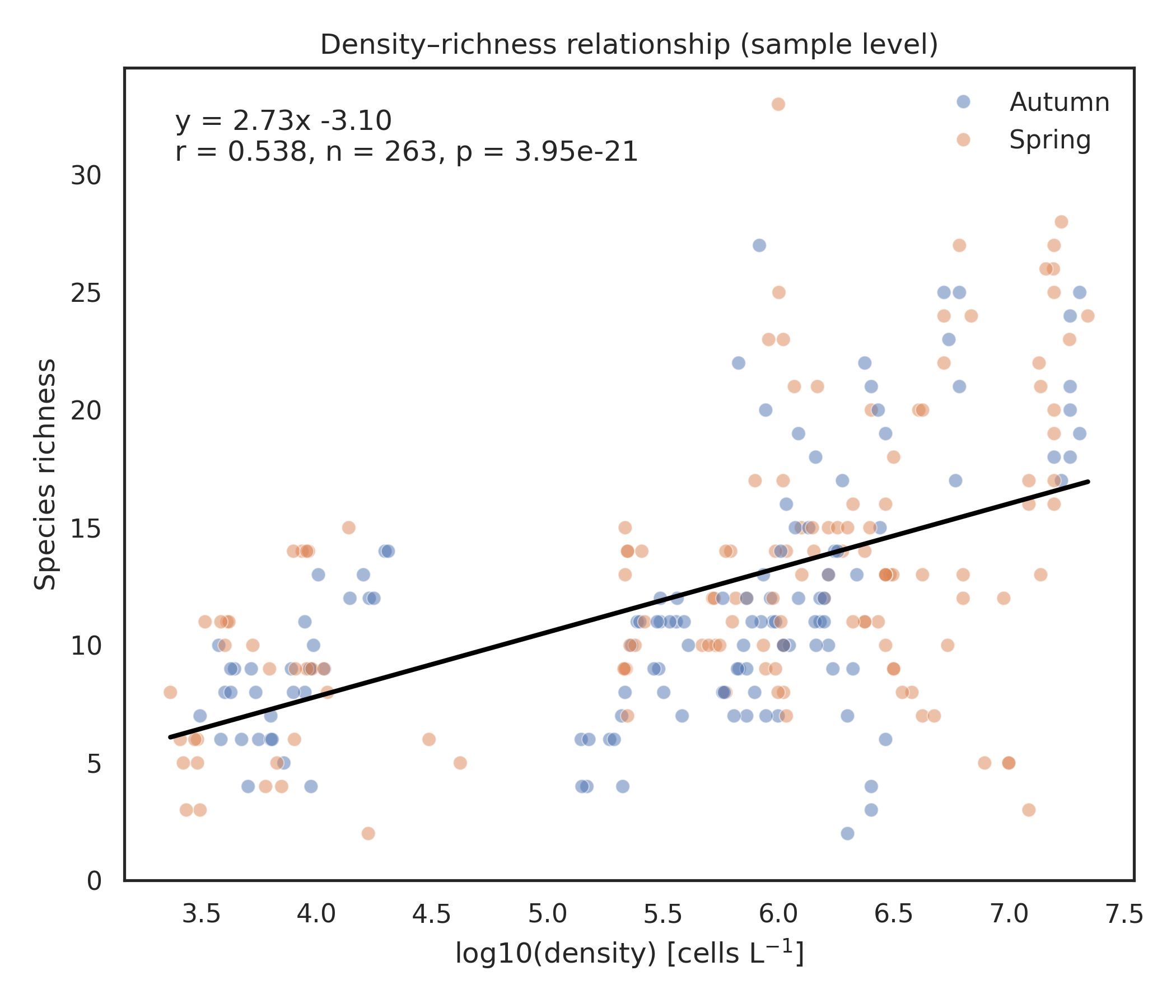
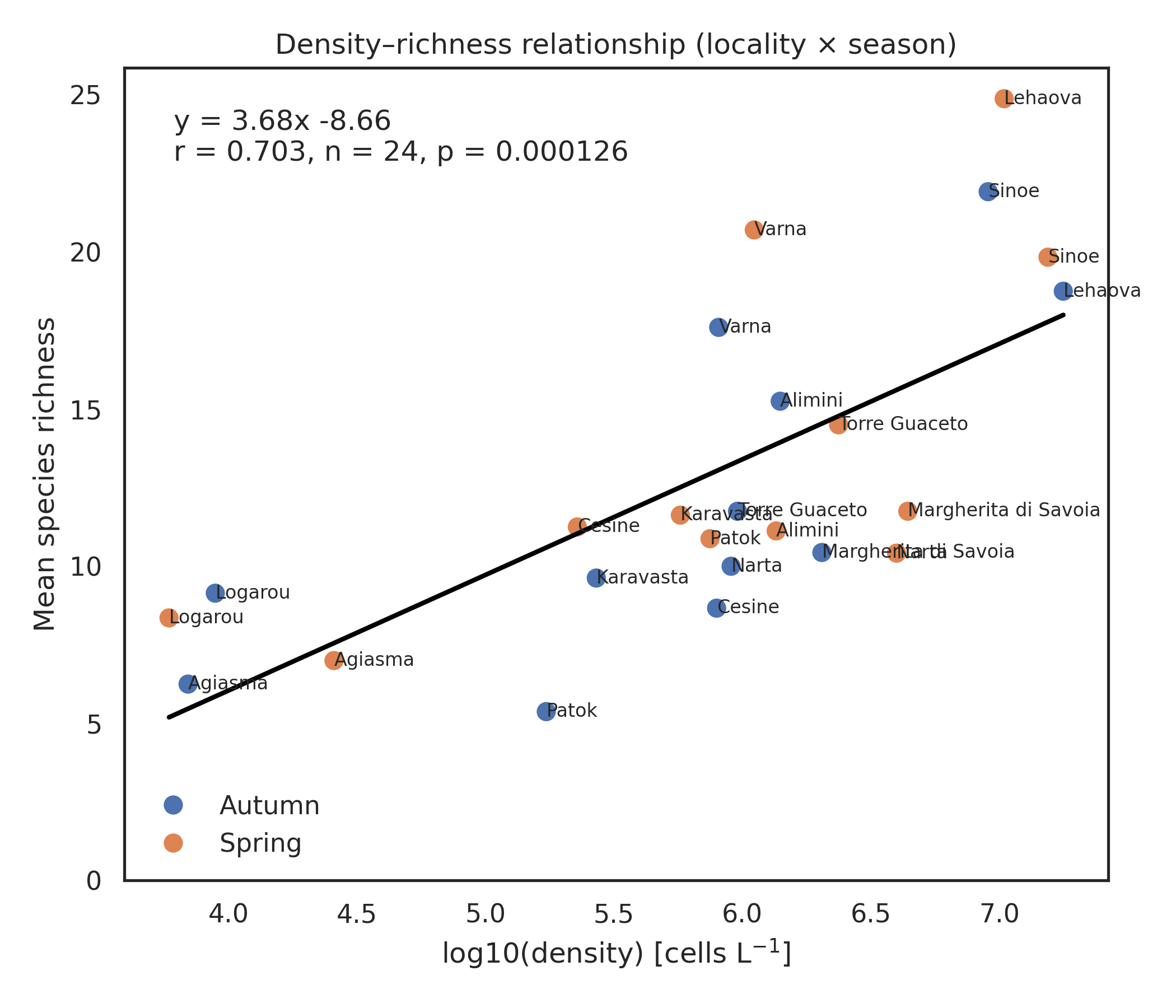
Figure 2. Relationships between phytoplankton density and species richness. (a) Sample-level (b) Ecosystem-level (locality × season).
Community similarity and multivariate comparisons
Phytoplankton community composition exhibited marked differences among the studied ecosystems, while seasonal effects were comparatively weaker. Morisita–Horn similarity values revealed a clear spatial structure, with high similarity among lagoons located in the same geographical regions and much lower similarity between northern Adriatic, Ionian and Black Sea systems (Figure 3a). Several ecosystems, including Agiasma, Logarou and Sinoe, formed well-defined clusters with high internal similarity, whereas others (e.g. Karavasta, Torre Guaceto) showed broader internal variability. The nMDS ordination based on Bray–Curtis dissimilarities further supported these patterns (stress = 0.1953), showing distinct grouping of communities by locality (Figure 3b). Samples belonging to each lagoon were generally clustered together, indicating strong ecosystem-specific assemblages. Spring and autumn samples from the same locality tended to overlap considerably, suggesting that spatial differences dominate over seasonal variation in shaping community structure. Only a few lagoons exhibited moderate seasonal shifts in ordination space, reflecting local hydrological or environmental dynamics. SIMPER analysis indicated that only a small fraction of taxa drove most differences in community composition among lagoons. The top five contributors explained on average ~28% of between-lagoon dissimilarity (range: 15–40%). The most influential groups included diatoms (e.g. Ceratoneis closterium, Cyclotella caspia), dinoflagellates (e.g. Prorocentrum cordatum), and green algae (e.g. Scenedesmus, Crucigenia), although their relative importance varied markedly among ecosystems.
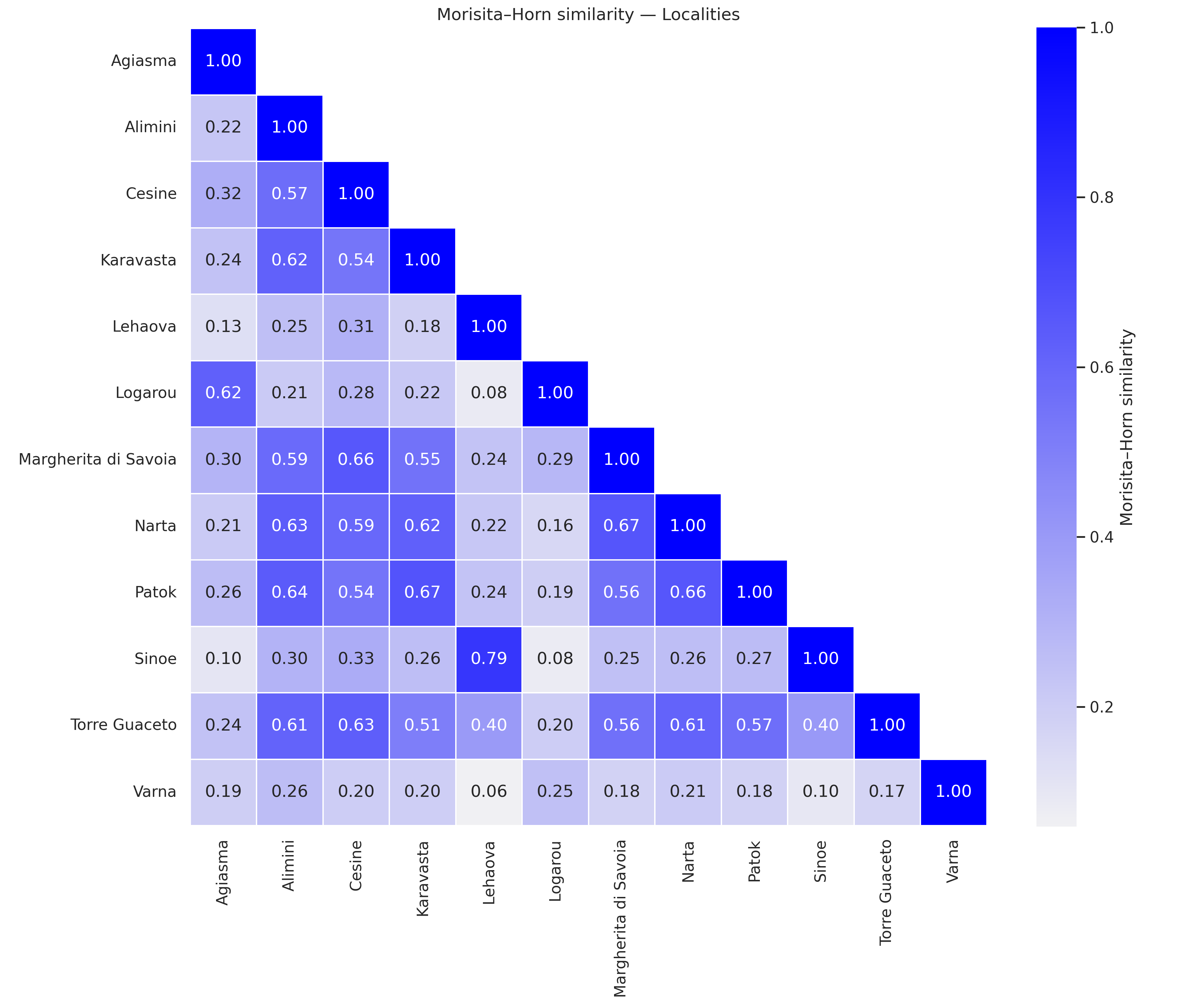

Figure 3. a) Morisita–Horn similarity matrix among ecosystems. b) nMDS ordination (Bray–Curtis) of phytoplankton community composition.
Relationships between phytoplankton density, richness and environmental variables
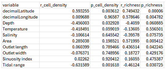
Univariate regressions revealed contrasting effects of environmental gradients on phytoplankton structure (Table 1). Phytoplankton density increased significantly with latitude (r = 0.59, p < 0.01) and declined with depth (r = –0.46, p < 0.05) and temperature (r = –0.42, p < 0.05). No significant relationships were found with salinity, outlet morphology, area, or sinuosity. Species richness showed a different response pattern, increasing with latitude (r = 0.75, p < 0.001) and outlet length (r = 0.44, p < 0.05), while decreasing significantly with tidal range (r = –0.46, p < 0.05) and salinity (p ≈ 0.07; marginal). No meaningful associations emerged with outlet width, sinuosity or temperature. Environmental controls on community turnover were examined by correlating Bray–Curtis dissimilarity with environmental distances computed separately for each abiotic variable (Figure 4). Phytoplankton taxonomic dissimilarity increased strongly with geographic gradients, showing significant positive correlations with longitude (r = 0.59, p < 0.001) and latitude (r = 0.52, p < 0.001). Morphological differences among lagoons also contributed: outlet length (r = 0.43, p < 0.001), lagoon area (r = 0.31, p < 0.001), and outlet width (r = 0.30, p < 0.01) were all positively related to taxonomic dissimilarity. Depth had a weaker but still significant effect (r = 0.15, p < 0.05), whereas salinity and sinuosity index showed no significant association, indicating that structural turnover was more strongly driven by spatial gradients and hydromorphological constraints than by local physicochemical conditions.
Table 1. Pearson correlations between individual environmental variables and phytoplankton density and species richness.

Technical notes
All analytical steps developed for this case study were adapted specifically for the characteristics of the present dataset, but all variables, parameters and analytical procedures can be easily adjusted for other systems or case studies as needed.
References
The analytical workflow applied here builds upon and extends the approaches developed in earlier works:
Vadrucci, M. R., Sabetta, L., Fiocca, A., Mazziotti, C., Silvestri, C., Cabrini, M., … & Basset, A. (2008). Statistical evaluation of differences in phytoplankton richness and abundance as constrained by environmental drivers in transitional waters of the Mediterranean basin. Aquatic Conservation: Marine and Freshwater Ecosystems, 18(S1), S88–S104.
Vadrucci, M. R., Stanca, E., Mazziotti, C., Umani, S. F., Georgia, A., Moncheva, S., … & Basset, A. (2013). Ability of phytoplankton trait sensitivity to highlight anthropogenic pressures in Mediterranean lagoons: A size spectra sensitivity index (ISS-phyto). Ecological Indicators, 34, 113–125.
Sangiorgio, F., Basset, A., Pinna, M., Sabetta, L., Abbiati, M., Ponti, M., … & Reizopoulou, S. (2008). Environmental factors affecting Phragmites australis litter decomposition in Mediterranean and Black Sea transitional waters. Aquatic Conservation: Marine and Freshwater Ecosystems, 18(S1), S16–S26.